Workstream 1 Individual contribution
Continuous-time STGNNs for normal and extreme weather
Praise Jaravani — crossing the spatial prior with the temporal formulation, and asking whether average accuracy says anything about accuracy on extremes.
Research question
Spatio-temporal graph neural networks achieve strong average-case accuracy for station-level weather forecasting. Two things stayed untested: their behaviour on the extreme events that symmetric training losses smooth away, and how far ahead their forecasts remain skillful.
This workstream benchmarks MTGODE — a continuous-time neural-ODE STGNN and, to the best of our knowledge, the first applied to weather forecasting — against STGODE, AGCRN and CLCRN, crossing the spatial prior (learned versus geometric) with the temporal formulation (discrete versus continuous) in a 2×2 design over 32 SAWS stations. Evaluation spans 48-hour regression stratified by extremes, and extreme-event detection under calendar- and hour-relative percentile labels.
Contributions
- The first application of MTGODE — and of learned-adaptive-graph neural ODEs generally — to meteorological forecasting, on an irregular station network.
- A 2×2 comparison of spatial prior against temporal formulation on South African station data under a single pipeline, extending the Davidson–Gaibie lineage to 48-hour horizons.
- An extreme-event detection formulation that extends ETCCDI percentile indices to hourly resolution through calendar- and hour-relative thresholds, with pre-registered naive baselines and decision rules, removing by construction the calendar signal that static thresholds concede to any climatology-aware classifier.
- WeatherFLOW, a reproducible benchmarking framework integrating four STGNN families under a single training and evaluation harness, with implementation-fidelity audits reported.
The 2×2 design
The four architectures were not chosen for coverage. They instantiate every combination of the two properties that distinguish them, so that each axis can be read against the other rather than confounded with it.
| Spatial prior \ Temporal | Discrete time | Continuous time (neural ODE) |
|---|---|---|
| Learned adaptive graph | AGCRN | MTGODE |
| Geometric graph | CLCRN | STGODE |
Holding everything outside those two axes fixed — same tensors, same splits, same loss, same optimiser, same seeds, same evaluation — means a difference between cells is attributable to the design, and the interaction between the axes becomes measurable rather than assumed. That interaction turned out to be the main result.
Method
Two tasks
Phase 1 is deterministic multi-step regression: a 12-hour input window maps to a joint 48-hour forecast over all stations, reported at six sub-horizons by truncation of the direct forecast. Targets are temperature, surface pressure, relative humidity and wind speed; all six recorded variables are available as input.
Phase 2 is extreme-event detection. The ground truth is whether an observation exceeds a threshold conditioned on station, variable, day-of-year and hour-of-day — the 95th percentile of training observations pooled over a ±7-day, ±1-hour window that wraps at year and day boundaries. This extends the ETCCDI moving-calendar-window convention to hourly resolution, with the day window widened from five days to seven so that a six-year baseline clears the roughly 200 samples a stable 95th-percentile estimate needs.
Each model's output is mapped to one logit per station, horizon step and label variable, and trained as a multi-label classifier with weighted binary cross-entropy. Training positive rates are 4–5% for temperature, humidity and wind speed but about 0.28% for precipitation, giving a precipitation weight near 350. STGODE sits out Phase 2 — its univariate output head is incompatible with the multi-label path.
- Campaign
- 4 models × 4 targets × 10 seeds = 160 regression runs; 3 models × 10 seeds = 30 detection runs; 190 runs total
- Seeds
- {42…51}, with full seeding of Python, NumPy and PyTorch
- Input window
- 12 hours
- Horizon
- 48 hours, reported at 3, 6, 9, 12, 24, 48
- Loss
- mean absolute error; Adam; per-paper learning-rate schedules; gradients clipped at 5.0; early stopping patience 15
- Hardware
- NVIDIA L40S, UCT ICTS HPC
Why the labels are calendar-relative
A fixed per-station percentile absorbs a variable's annual cycle, so a classifier told nothing but the calendar-hour exceedance frequency can score far above chance. Measured directly: under static thresholds such a classifier reaches 5.98× prevalence on temperature. Under the calendar- and hour-relative scheme it falls to no skill on three variables (0.87 to 0.93) and only just above on precipitation. The labels therefore concede no calendar signal, and the detection results are not an artefact of seasonality.
Running the authors' code
Upstream repositories are vendored at pinned commits and never modified; each integration is an adapter wrapping the published code behind a common interface. An external implementation audit of the MTGODE integration preceded all reported runs and found three defects, each corrected before relaunch: the adjoint backward pass structurally excluded the graph learner's parameters from gradient flow, so the learned adjacency stayed at its random initialisation; the graph-learner embedding dimension had been conflated with the convolutional width; and the spatial vector field was implemented at half the required magnitude. No result produced before these corrections is reported.
One inherited hyperparameter also needed repair. Gaibie et al.'s AGCRN learning rate of 0.01 exceeds the ceiling of the original authors' published search range and diverged on this network, with best validation at epoch 1. A pre-registered single-seed diagnostic selected the original published optimum of 0.003, a 42% reduction in validation MAE.
Findings
Result 1 · Continuous time transfers, conditionally
MTGODE attains the lowest error on three of four variables and is inseparable from CLCRN on surface pressure — the first demonstration that a continuous-time graph model works on an irregular station network. But STGODE is continuous-time too and is the weakest of the four, so continuity alone does not carry the result.
Result 2 · Neither design axis helps alone
The interaction dominates. Moving from discrete to continuous time lowers error under a learned adaptive graph and raises it under a geometric prior — the lines cross on every variable. The interaction is negative on all four, from −3.28% to −5.19% of the four-cell mean, and exceeds either marginal effect. The pattern is diagonal rather than marginal: the cells pairing a learned graph with continuous time, and a geometric prior with discrete recurrence, both fall below each variable's mean, while the two crossed pairings fall above it.
Result 3 · All four models smooth the tails
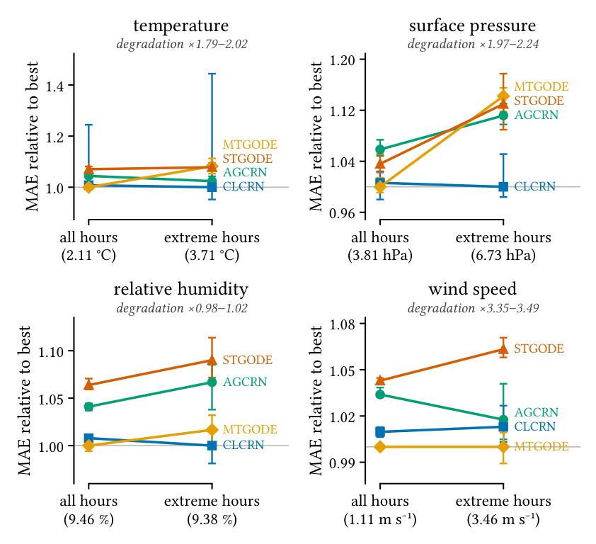
Error degrades by up to a factor of 3.5 on extreme hours, and the model most accurate on average is not the model most accurate on extremes. On temperature, AGCRN attains the lower extreme-regime MAE in 90% of cross-pairs against MTGODE and 93% against STGODE. Mean error is the wrong criterion for selecting an extreme-event forecaster.
Result 4 · Accuracy is not bought with scale
The most accurate model is also among the cheapest, at 138,096 parameters against 1,663,104 for the weakest. CLCRN, the smallest of the four, separates from the far larger STGODE on all four variables. Parameter count and inference speed do not track one another either.
Forecast validity
The valid forecast horizon is the last lead at which pooled NRMSE stays at or below a threshold ε, with all NRMSE normalised by the frozen training-split standard deviation so that ε = 1.0 marks climatology-equivalent error.
| Model | ε = 0.3 | ε = 0.5 | ||||||
|---|---|---|---|---|---|---|---|---|
| t2m | sp | rh | ws | t2m | sp | rh | ws | |
| AGCRN | 2.0 | 0 | 1.0 | 0 | 26.2 | 0 | 5.2 | 0.9 |
| CLCRN | 2.6 | 0 | 1.0 | 0 | 25.6 | 0 | 6.6 | 1.0 |
| MTGODE | 3.0 | 0 | 1.0 | 0 | 29.2 | 2.6 | 7.0 | 1.0 |
| STGODE | 1.9 | 0 | 1.0 | 0 | 25.1 | 0.4 | 4.7 | 1.0 |
| Persistence | 1 | 0 | 0 | 0 | 2 | 3 | 1 | 1 |
| Climatology | 0 | 0 | 0 | 0 | 0 | 0 | 0 | 0 |
At the looser threshold the horizon recovers the mean-error ordering on temperature and humidity but not on pressure, where CLCRN reaches zero hours yet ties for lowest MAE, and persistence outlasts every model. The pre-registered threshold is too strict to arbitrate between the architectures on this data — a reportable negative result rather than a tuning opportunity.
Seed stability and the divergent run
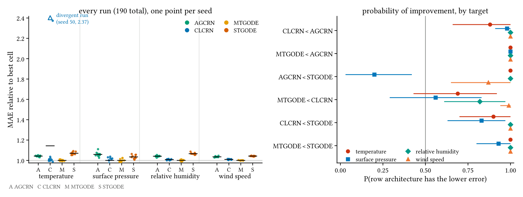
Fifteen of the sixteen (model, target) regression cells are stable under reinitialisation, with coefficients of variation of test MAE from 0.18% to 3.02%. Surface pressure carries the highest variation for every model; wind speed, where the signal is strongest, converges to nearly the same error across runs.
The sixteenth cell is the exception, and it is reported as a finding rather than cleaned away. On temperature, CLCRN's seed 50 converged to the training mean: its validation loss never fell below its first-epoch value and its test error equals the climatological forecast's — 5.003 against 5.005 °C. The failure reproduced under the same seed. It is one run in 190 and it is retained in every reported statistic.
Its effect is the reliability result. It inflates that cell's standard deviation to ±0.912 against ±0.013 to 0.029 elsewhere, and lifts the cell mean by 0.29 °C — about twice the widest gap between converged architectures (0.148 °C). It struck the strongest-signal variable. Under the previous study's three-run budget it would have been a third of a cell, and it flips the sign of the mean-based temperature interaction, which is why the factorial analysis rests on the interquartile mean rather than the raw mean. That the failed run is a CLCRN run is consistent with CLCRN's authors naming training instability an open problem of the method, though one run cannot establish a rate.
| Comparison | t2m | sp | rh | ws |
|---|---|---|---|---|
| MTGODE > CLCRN | .69 [.43, .91] | .56 [.28, .83] | .82 [.61, .97] | .99 [.94, 1.0] |
| MTGODE > AGCRN | 1.0 [1.0, 1.0] | 1.0 [1.0, 1.0] | 1.0 [1.0, 1.0] | 1.0 [1.0, 1.0] |
| MTGODE > STGODE | 1.0 [1.0, 1.0] | .93 [.80, 1.0] | 1.0 [1.0, 1.0] | 1.0 [1.0, 1.0] |
| CLCRN > AGCRN | .88 [.67, 1.0] | .98 [.91, 1.0] | 1.0 [1.0, 1.0] | 1.0 [1.0, 1.0] |
| CLCRN > STGODE | .90 [.70, 1.0] | .83 [.63, .97] | 1.0 [1.0, 1.0] | 1.0 [1.0, 1.0] |
| AGCRN > STGODE | 1.0 [1.0, 1.0] | .20 [.04, .42] | 1.0 [1.0, 1.0] | .87 [.65, 1.0] |
Across the 40 (target, seed) cells MTGODE takes first place in 31 and CLCRN in the other 9; no other model leads anywhere. The bottom of the ranking is reproducible and the top is not on temperature and pressure.
Where the hard stations are
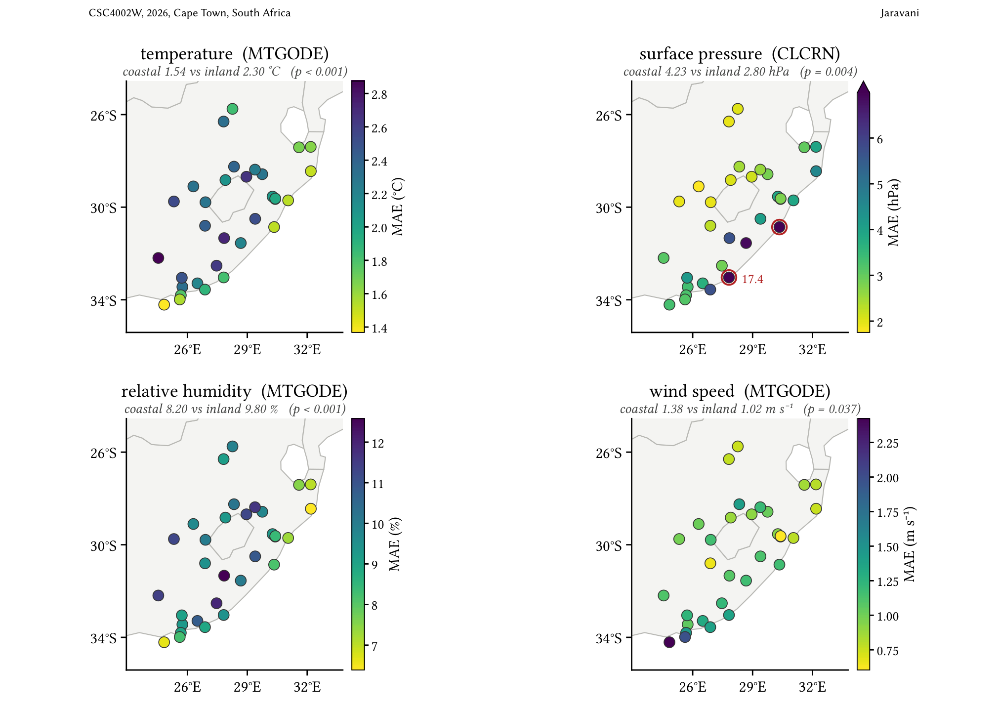
Station difficulty is a property of the sites, not the architectures: the four models rank the 32 stations near-identically, with per-station error correlations of 0.98 to 1.00 on every variable. The coastal–inland contrast reverses by variable — temperature and relative humidity are forecast more accurately at the coast, wind speed and surface pressure less so — and all four differences are significant.
Case study: the December 2024 heatwave
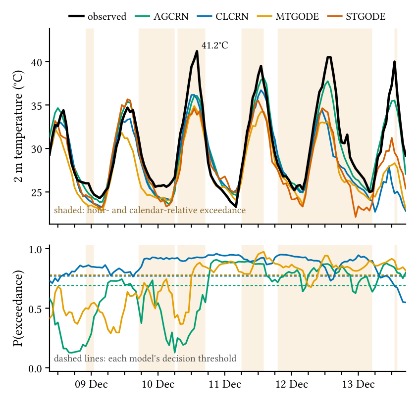
The aggregate extreme results are reproduced on a single named event at Makatini station, at 24-hour lead. The case study shows the mechanism directly: each model follows the diurnal shape of the event but flattens its amplitude, so error concentrates exactly where the observation is most extreme. Detection recall collapses as lead grows.
This is the double-penalty behaviour of a smooth predictor under a squared-error objective, compounded by the scarcity of tail samples that leaves the high quantiles under-fit. The deficit sits in the training objective, not in the architecture.
Discussion
Continuous-time formulations work when the graph is learned
A claim about either design axis is conditional on the other. This is consistent with the MTGODE authors' positioning of their model against STGODE on continuous temporal aggregation, without isolating it — STGODE's cell also differs in spatial prior, takes a single Euler step, and won its hyperparameter search at the grid bound on three of five knobs, which makes its result a lower bound on that corner of the design rather than a tuned optimum. Where the MTGODE authors report their model's edge as largest at long horizons, here it is largest at short lead.
No single criterion selects one architecture
On average error, on forecast validity at the looser threshold, and on detection ranking, MTGODE leads. In the tail, a discrete-recurrence model has the lower regression error on three of four variables. Capacity buys none of it. The criteria fall into two families — average-case skill and tail amplitude — that do not agree, so the choice of model follows the intended use rather than a single ranking.
The results transfer in scale but not in order
Gaibie et al. rank AGCRN ahead of CLCRN on temperature, humidity and wind speed from three runs without dispersion; here CLCRN separates from AGCRN on all four, the two studies agreeing only on pressure. Several factors are confounded — the eastern rather than Cape network, the inherited optima, and three runs against ten seeds. Pressure is the sharpest contrast: most predictable in the earlier study's normalised units but least predictable here in physical ones, because min–max normalisation over a wide altitude range shrinks pressure error by construction. What transfers is the size of the differences, not their order.
Static exceedance thresholds are not comparable across variables
Because a fixed per-station percentile absorbs a variable's calendar cycle, a seasonal classifier scores far above chance under it, and by an amount that differs sharply by variable — 5.98× prevalence on temperature against 2.44× on precipitation. The calendar- and hour-relative scheme removes that signal, restoring no skill on three of the four variables.
Limitations and future work
Evaluation uses a single chronological hold-out rather than walk-forward validation, and hyperparameter selection is asymmetric — inherited optima for the baselines, an Optuna search for the continuous-time models. The network is confined to the summer-rainfall east. The extreme-event picture is narrower still: it rests on one named event, on single-hour labels with no duration structure, and on a non-stationary tail that a frozen decision threshold cannot track — test positive rates run about 1.6× the training rate on temperature and 2.8× on humidity.
Each limit points to a next step. A single architecture whose spatial prior and temporal formulation switch independently would turn the interaction into a controlled effect rather than one confounded with other differences between the cells. A tail-weighted or probabilistic objective would address the smoothing every model shows — the remedy is the loss, not a larger model. Duration-aware labels with recalibrated thresholds would suit operational use.
Documents
- Final paper Continuous-Time and Discrete Spatio-Temporal Graph Neural Networks for Normal and Extreme Weather Prediction on South African Station Data
- Literature review Weather Flow Prediction Using Spatial-Temporal Graph Neural Networks: A Literature Review
- WeatherFLOW source code The whole framework — preprocessing, training harness and evaluation suite — with this workstream's models under models/continuous_time/ and the shared baselines under models/baselines/.
- Project poster Joint deliverable covering all three workstreams.
- Project proposal Joint proposal by Chikwanha, Fuyana and Jaravani, setting out how the study would be conducted.