Workstream 2 Individual contribution

Diffusion-based STGNNs for weather prediction

Génevieve Chikwanha — whether generating a distribution of possible futures beats predicting a single one, and what actually separates two diffusion models from each other.

Research question

Conventional STGNNs are deterministic: they emit one number per station per hour and so cannot express how uncertain that number is. Diffusion models offer an alternative — learn to reverse a noising process, and the forecast becomes a sample from a distribution, so repeating the process yields many plausible futures. The approach has shown promise on traffic and urban sensor data, but it was not clear whether its advantages transfer to weather forecasting, and particularly to an irregularly distributed station network.

This workstream evaluates DiffSTG and USTD against the deterministic AGCRN and CLCRN baselines on the same 32 SAWS stations, scoring both point accuracy (MAE, RMSE) and distributional quality (CRPS) over horizons to 48 hours.

Contributions

An empirical comparison of two diffusion-based STGNNs against established deterministic STGNNs for weather forecasting on South African station data.
Evaluation of both point and probabilistic forecasting performance across four weather variables and horizons to 48 hours, using MAE, RMSE and CRPS.
Analysis of forecasting error across time and space — node-level performance and the relationship between error, station elevation and local weather variability.

The two diffusion models

Both learn to reverse a noising process; they differ in what the denoiser sees while doing it. That difference turns out to decide the result.

Diffusion Predefined graph

DiffSTG

Wen et al. — diffusion over spatio-temporal graphs

Combines the diffusion process with a UGnet denoiser: temporal convolutional blocks model temporal dependency and graph convolutional blocks propagate between spatially connected nodes. During training the future target is progressively corrupted with noise while the historical observations condition the denoising; at inference the process runs in reverse from random noise. It is explicitly non-autoregressive, generating the whole horizon at once.

In this implementation the history is the conditioning sequence, the same predefined distance-based adjacency is used throughout, and no additional covariates are supplied.

Diffusion Encoder + covariates

USTD

Hu et al. — unified spatio-temporal diffusion

Puts a deterministic encoder in front of the diffusion. Graph convolutions extract a representation of the historical spatio-temporal context, and a diffusion Transformer then denoises the noisy future using self-attention across stations and time. Spatial position enters through Laplacian positional encodings derived from the graph; temporal position is supplied separately.

In this implementation the history and covariates pass through a Graph WaveNet encoder with the predefined adjacency, and the result conditions the Transformer alongside time of day, day of year and station height, supplied for both historical and future steps.

Method

The SAWS supply covered 60 automatic weather stations across the Free State, Gauteng, KwaZulu-Natal and the Eastern Cape. Twenty-eight exceeded the 10% missingness threshold and were excluded, leaving 32 — 13 in the Eastern Cape, 12 in KwaZulu-Natal, 5 in the Free State and 2 in Gauteng. Remaining gaps were filled by inverse-distance weighting, which estimates a missing value as a distance-weighted average of concurrent observations at neighbouring stations.

Four of the six recorded variables were modelled, excluding rainfall and wind direction. Each variable was trained separately and univariately: the input tensor was sliced per feature, so a model forecasting temperature sees only temperature history. This differs from the continuous-time workstream, which supplies all six variables as input while predicting one — a difference worth holding in mind when comparing the two sets of numbers.

Observations: 87,672 hourly timesteps × 32 stations × 4 features = 11,222,016 observations
Split: chronological 60 / 20 / 20 — train 2016–2021, validate 2022–2023, test 2024–2025
Normalisation: z-score, mean and standard deviation from the training set only
Seeds: 3 — 2024, 2025, 2026
Samples: 8 per diffusion run, averaged for comparison with the deterministic baselines
Training: MAE objective, Adam; max 50 epochs for baselines, 300 for diffusion models; early stopping patience 15
Tuning: Tree-structured Parzen Estimator, 30 trials of 30 epochs; first 10 trials random, remaining 20 guided
Hardware: NVIDIA A100, UCT ICTS HPC

Metrics

MAE and RMSE are reported together because they weight the error distribution differently — RMSE's sensitivity to large errors makes it the more informative of the two when the question concerns extremes. CRPS is added for the diffusion models: it scores the compatibility of a whole predictive distribution with the observation, which MAE and RMSE cannot do because they score only a point.

Findings

Result 1 · Diffusion did not beat deterministic

CLCRN is the best point forecaster on every variable and both metrics. It improves on AGCRN by about 4% on humidity, 11% on pressure and 2% on temperature, and beats USTD by 3–10% across the board. Diffusion-based forecasting does not inherently improve weather prediction on this data.

Result 2 · DiffSTG was the weakest of the four

Highest MAE and RMSE on every single variable. Its pressure MAE is roughly 47% higher than USTD's and 64% higher than CLCRN's; on humidity and temperature it trails the others by 5–17%. This is consistent with its own authors' results, where it also failed to surpass its deterministic baselines.

Result 3 · USTD was competitive

It tracks AGCRN within 3% on MAE for every variable — the largest gap being wind speed, where AGCRN is 2.23% lower — and beats AGCRN by 12.93% on pressure RMSE. It also produced better probabilistic forecasts than DiffSTG on three of four variables.

Result 4 · The gap is in the conditioning, not the paradigm

Both models are diffusion models and both are non-autoregressive, so neither property explains a 47% difference. What separates them is that USTD denoises a representation that a deterministic encoder has already structured, and conditions on time of day, day of year and station height. The ablation confirms it directly.

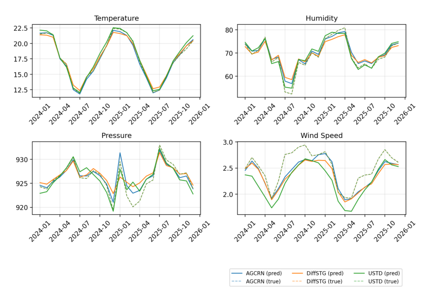
Four line charts showing each model's monthly predicted values against the ground truth for temperature, humidity, pressure and wind speed across the 2024 to 2025 test period. All models track the seasonal shape; DiffSTG deviates furthest from the observed trajectory. — **Predictions against ground truth across the test period.** DiffSTG captures the broad temporal structure of temperature and wind speed but sits further from the observed trajectory than the other three, suggesting a limitation in representing how the forecast evolves across the full horizon rather than a failure to learn the signal at all. Figure 4, Chikwanha (2026).

Why conditioning decides it

Learning the full shape of a probability distribution, in order to give reliable uncertainty ranges, requires more information than learning a direct mapping from an input to a single output. A strong conditional representation gives the generative step a better foundation — particularly when the available observations alone do not fully describe the state of the atmosphere, which at 32 irregularly spaced stations they certainly do not.

Non-autoregressive generation is not the culprit. Both diffusion models are non-autoregressive, yet only one underperforms; and TimeDiff, which is also non-autoregressive, performs strongly precisely because it adds autoregressive initialisation and future-mixup conditioning. What matters is how temporal dependencies are encoded before or during generation, not whether the forecast is produced in one shot.

The ablation makes the argument empirically. Stripping USTD's exogenous covariates raises its RMSE on every variable, and on pressure — the variable most tied to station altitude — the error rises by 45%.

**USTD ablation.** Test RMSE with all exogenous covariates, against RMSE with none. Station height is one of the covariates removed.
Variable	All covariates	No covariates	Deterioration
Surface pressure (hPa)	9.117	13.230	+45.1%
Temperature (°C)	2.974	3.411	+14.7%
Wind speed (m s⁻¹)	1.647	1.737	+5.5%
Relative humidity (%)	13.867	14.523	+4.7%

Spatial and elevation patterns

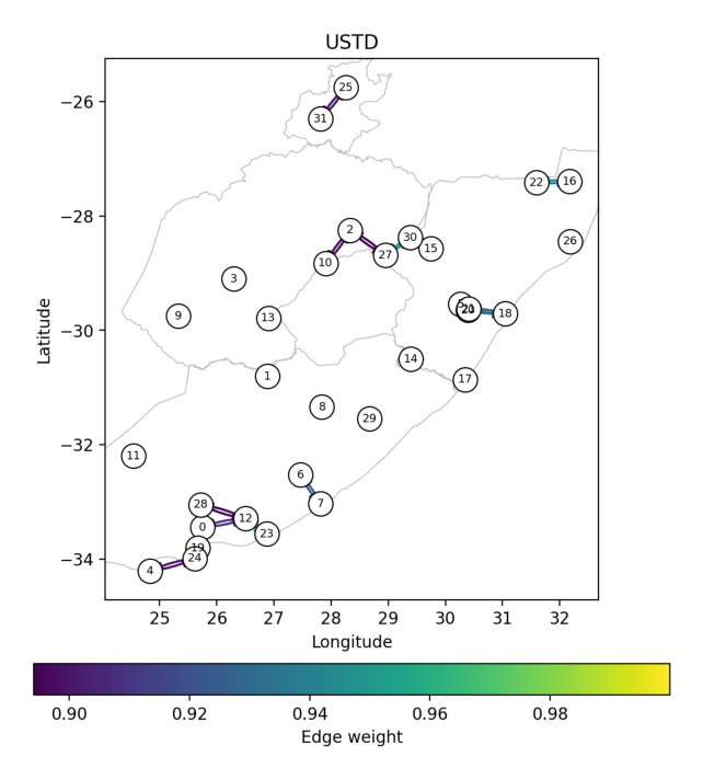
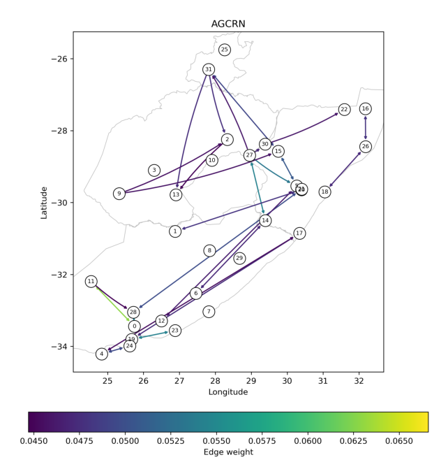
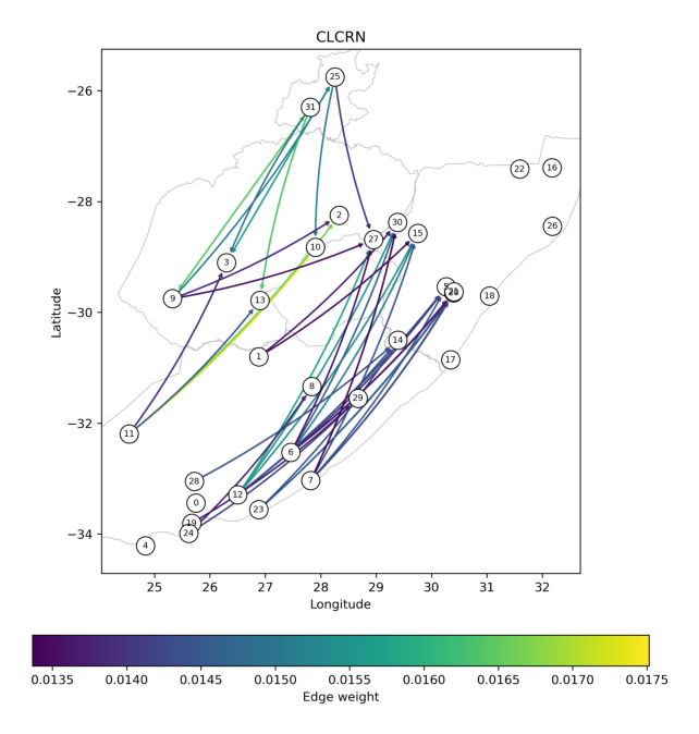
Following the earlier studies in the lineage, the 40 highest-weight edges of each model's adjacency matrix were plotted on a map of the covered provinces, so that what each model believes about the network can be inspected directly.

The predefined matrix used by DiffSTG and USTD is built from weighted distance and is symmetric, so every edge is bidirectional and the strongest connections are simply the geographically closest ones — it focuses on local neighbourhoods and clusters accordingly. AGCRN and CLCRN, which do not use a predefined adjacency, learn visibly more complex and longer-range structure.

Map of the eastern provinces with 32 numbered station nodes; the 40 strongest edges of the predefined adjacency matrix connect only geographically adjacent stations in tight local clusters. — **Predefined adjacency.** Used by DiffSTG and USTD — local, symmetric, distance-driven. Figure 5, Chikwanha (2026).

Map of the same station network showing AGCRN's learned adjacency as directed arrows, including many long-range connections between distant stations. — **AGCRN's learned graph.** Directed, and willing to connect distant stations. Figure 6, Chikwanha (2026).

Map of the same station network showing CLCRN's learned spatial node embeddings as directed arrows between stations. — **CLCRN's learned structure.** Conditioned on geodesic distance and orientation. Figure 7, Chikwanha (2026).

Variability, not just position, drives error

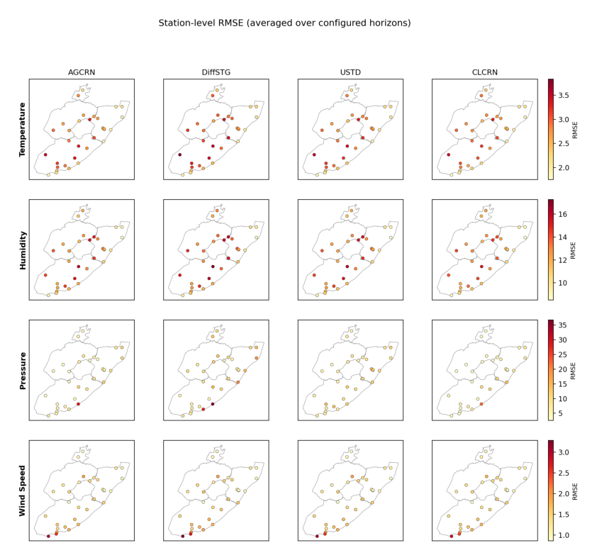
Geographic proximity does not capture everything that matters. Node 9, the least stable station in the dataset with a temperature standard deviation of 8.73 and a range of 50.8 °C (−9.9 to 40.9), produces the highest MAE and RMSE for all four models. Coastal nodes are among the most stable and among the best forecast on temperature. For pressure the pattern breaks: DiffSTG performs particularly poorly along the KwaZulu-Natal and Eastern Cape coastlines despite those stations being relatively stable, so stability alone does not explain pressure error.

Elevation

Node 25 consistently shows higher temperature error than its close neighbour node 31, across all four models — so proximity alone does not explain the difference. USTD achieves the lowest error at these nodes and AGCRN also performs well. The same pattern recurs at three high-elevation nodes near the Free State–KwaZulu-Natal and Free State–Lesotho borders, and at an isolated Eastern Cape station. Since AGCRN learns an adaptive adjacency and USTD is conditioned on station height, both have a route to information that distance alone does not carry — which is consistent with, though not proof of, the elevation explanation.

A grid of four maps of the covered provinces, one per model, with node-specific RMSE values overlaid on each station position. — **Node-level RMSE by model.** Stations that are hard for one model are generally hard for all of them, but the pressure maps separate the models more than the other variables do. Figure 8, Chikwanha (2026).

Uncertainty and CRPS

The probabilistic results give a different view of the two diffusion models. Although USTD consistently produced lower MAE and RMSE than DiffSTG, its generated samples were visibly more dispersed, particularly for wind speed — so a narrower predictive distribution does not imply a more accurate point forecast. The central tendency of a generated distribution can be accurate even when individual samples span a wide range.

CRPS resolves the ambiguity. USTD achieves lower CRPS than DiffSTG on pressure, temperature and humidity, with the largest improvement on pressure (0.0060 to 0.0043). On wind speed it is worse (0.3745 to 0.4073) despite the slightly lower point error — there, the extra dispersion means the predictive distribution is less well matched to the observations. Sample spread is not itself a measure of uncertainty quality; whether dispersion helps depends on how well the resulting distribution represents what actually happened.

This matters for how probabilistic STGNNs should be judged. The motivation for diffusion-based forecasting was never purely point accuracy — it was the inability of conventional STGNNs to represent intrinsic uncertainty. On this data the diffusion formulation gave no consistent point-accuracy advantage, but USTD did give improved probabilistic performance on three of four variables. The value of a probabilistic model should be assessed on whether its predictive distributions are useful, not only on whether they reduce point error.

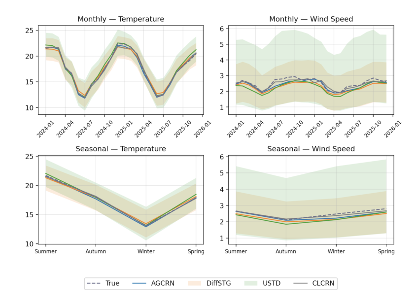
Two charts comparing predicted against true values for wind speed and temperature, with the eight individual samples generated by each diffusion model shown as a spread around the mean prediction. USTD's samples are visibly more dispersed for wind speed. — **The eight generated samples per diffusion model.** USTD's samples spread more widely, particularly on wind speed — which helps its CRPS on three variables and hurts it on the fourth. Figure 9, Chikwanha (2026).

Limitations and future work

Each weather variable was modelled independently and the network covers 32 stations across four provinces, so multivariate forecasting and larger, more geographically diverse networks are both open. Evaluation focused on overall forecasting error rather than performance during extreme weather, which would be a more practically relevant test of robustness — the continuous-time workstream takes that question up directly.

Inverse-distance weighting for missing observations may introduce bias by relying on spatial proximity rather than elevation or local topography, which the elevation results suggest matters here. The four models also differ in architecture and in available contextual inputs, so performance differences cannot be cleanly attributed to individual components; more controlled ablations would be needed to isolate the effects of spatial structure, temporal conditioning and exogenous variables. Finally, probabilistic evaluation was limited to the diffusion models, since the baselines produce point forecasts only — comparing against probabilistic versions of deterministic STGNNs, and assessing calibration during extreme events, would strengthen the comparison.

Documents

← Continuous-time workstream Lightweight workstream →